05 | Introduction to Optimization with Gurobi (gurobipy)

Linear Programming: Formulation and Solution Methods

Author

Affiliation

Mr. Ozan Ozbeker

Management Information Systems and Supply Chain

1 Overview

Linear Programming (LP) is a fundamental optimization technique that helps decision-makers allocate limited resources optimally. In this module, we’ll explore how to formulate linear programming models, identify their components, and solve them using both Excel Solver and Python with Gurobi.

After completing this module, you will be able to:

Identify the three key components of a linear programming model
Formulate linear programming models from problem descriptions
Determine whether a function is linear or nonlinear
Solve linear programming problems using graphical methods
Implement and solve LP models using Excel Solver
Implement and solve LP models using Python with Gurobi
Interpret the results of your optimization models

2 Introduction to Linear Programming

Linear Programming (LP) is a powerful optimization technique used to find the best outcome in mathematical models with linear relationships. LP has wide applications in business and supply chain management, including:

Production planning and scheduling
Resource allocation
Transportation and distribution problems
Financial portfolio optimization
Network flow problems

2.1 What Makes a Problem Suitable for Linear Programming?

A problem can be solved using linear programming if:

The objective (what you’re trying to maximize or minimize) can be expressed as a linear function
All constraints can be expressed as linear inequalities or equations
All variables can take non-negative values (in standard form)

2.2 Components of a Linear Programming Model

Every LP model consists of three essential components:

Decision Variables: What you’re trying to decide (usually denoted as $X_{1}$ , $X_{2}$ , etc.)
Objective Function: The goal you’re trying to maximize or minimize ( $p r o f i t$ , $c o s t$ , etc.)
Constraints: Limitations on resources or requirements that must be satisfied

2.3 Linear vs. Nonlinear Functions

A linear function has the form:

$y = a_{1} x_{1} + a_{2} x_{2} + . . . + a_{n} x_{n} + b$

Where:

$x_{1}, x_{2}, . . ., x_{n}$ are variables
$a_{1}, a_{2}, . . ., a_{n}, b$ are constants

In a linear function:

Variables appear only to the first power (no squares, cubes, etc.)
Variables don’t multiply or divide each other
There are no transcendental functions (log, sin, etc.) of variables

Examples of linear functions:

$y = 2.5 x + 5$
$y = - x + 5$
$y = 5$ (constant function)
$x = 5$ (can be rewritten as $1 x = 5$ )

Examples of nonlinear functions:

$y = 2 x^{2}$ (variables raised to powers other than 1)
$y = 3 x / (2 x + 1)$ (variables dividing each other)
$y = 3 x * (2 x + 1)$ (variables multiplying each other)

3 The Wyndor Glass Co. Problem

Let’s examine a classic LP problem that we’ll use throughout this module. The Wyndor Glass Company produces high-quality glass products in three plants and is considering launching two new products:

Aluminum-framed glass doors (Product 1)
Wood-framed windows (Product 2)

Each plant has a limited number of production hours available per week:

Plant 1: 4 hours available for Product 1 only
Plant 2: 12 hours available for Product 2 only
Plant 3: 18 hours available for both products

The company earns:

$3,000 profit per batch of Product 1
$5,000 profit per batch of Product 2

The problem: How many batches of each product should Wyndor produce weekly to maximize profit?

3.1 Formulating the Wyndor Glass LP Model

Decision Variables:
- $X_{1}$ = Number of batches of Product 1 (aluminum-framed doors)
- $X_{2}$ = Number of batches of Product 2 (wood-framed windows)
Objective Function:
- Maximize $Z = 3 X_{1} + 5 X_{2}$ (profit in thousands of dollars)
Constraints:
- Plant 1: $1 X_{1} + 0 X_{2} \leq 4$ (hours available in Plant 1)
- Plant 2: $0 X_{1} + 2 X_{2} \leq 12$ (hours available in Plant 2)
- Plant 3: $3 X_{1} + 2 X_{2} \leq 18$ (hours available in Plant 3)
- Non-negativity: $X_{1}, X_{2} \geq 0$ (can’t produce negative amounts)

This complete mathematical model represents our optimization problem.

4 Solving LP Models Graphically

For LP problems with two decision variables, we can solve them graphically by:

Plotting each constraint on a graph
Identifying the feasible region (the area that satisfies all constraints)
Finding the optimal solution at one of the corner points of the feasible region

4.1 Steps to Solve the Wyndor Glass Problem Graphically:

Plot the constraints:
- Plant 1: $X_{1} \leq 4$ (vertical line at $X_{1} = 4$ )
- Plant 2: $X_{2} \leq 6$ (horizontal line at $X_{2} = 6$ )
- Plant 3: $3 X_{1} + 2 X_{2} \leq 18$ (line connecting points $(6, 0)$ and $(0, 9)$ )
- Non-negativity: $X_{1} \geq 0$ and $X_{2} \geq 0$ (the positive quadrant)
Identify the feasible region:
- The region bounded by these lines forms a polygon. Any point inside this polygon represents a feasible solution.
Find the optimal solution:
- The optimal solution will be at one of the corner points of the feasible region
- For a maximization problem, we want the corner point that gives the highest value of the objective function

Let’s calculate the objective function value at each corner point:

Corner Point	$X_{1}$	$X_{2}$	$Z = 3 X_{1} + 5 X_{2}$
(0,0)	0	0	0
(4,0)	4	0	12
(0,6)	0	6	30
(2,6)	2	6	36

The optimal solution is $X_{1} = 2$ , $X_{2} = 6$ , which gives a maximum profit of $36,000.

4.2 Using Level Curves to Find the Optimal Solution

Another approach is to use level curves of the objective function:

Draw the level curve $Z = 3 X_{1} + 5 X_{2} = C$ for some value of $C$
Increase $C$ until the level curve is about to leave the feasible region
The last point of contact is the optimal solution

This graphical method helps visualize how the optimal solution is found, though it becomes impractical for problems with more than two variables.

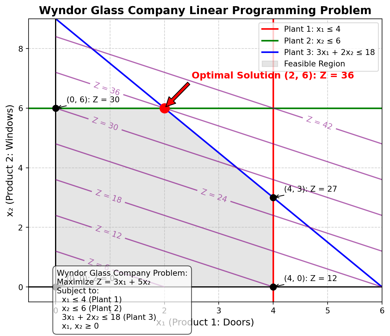
4.3 Visualization of the Wyndor Glass Problem

Let’s visualize the solution to better understand the constraints and optimal point:

Code

import matplotlib.pyplot as plt
import numpy as np

# Create a new figure with a specific size for better visibility
plt.figure(figsize=(7, 6))

# Define the range for x and y axes
x_range = np.linspace(0, 6, 100)
y_range = np.linspace(0, 9, 100)

# Create a meshgrid for contour plotting
X, Y = np.meshgrid(x_range, y_range)
Z = 3 * X + 5 * Y  # Objective function: 3x₁ + 5x₂

# Plot the constraints
# Constraint 1: x₁ ≤ 4 (Plant 1)
plt.axvline(x=4, color='red', linestyle='-', linewidth=2, label='Plant 1: x₁ ≤ 4')

# Constraint 2: x₂ ≤ 6 (Plant 2)
plt.axhline(y=6, color='green', linestyle='-', linewidth=2, label='Plant 2: x₂ ≤ 6')

# Constraint 3: 3x₁ + 2x₂ ≤ 18 (Plant 3)
# Convert to y = mx + b form: y ≤ (18 - 3x₁)/2 = 9 - 1.5x₁
constraint3_y = lambda x: (18 - 3 * x) / 2
plt.plot(x_range, [constraint3_y(x) for x in x_range], 'blue', 
            linestyle='-', linewidth=2, label='Plant 3: 3x₁ + 2x₂ ≤ 18')

# Non-negativity constraints
plt.axhline(y=0, color='black', linestyle='-', linewidth=1.5)
plt.axvline(x=0, color='black', linestyle='-', linewidth=1.5)

# Define the vertices of the feasible region
feasible_region_x = [0, 0, 2, 4, 4]
feasible_region_y = [0, 6, 6, 3, 0]

# Shade the feasible region
plt.fill(feasible_region_x, feasible_region_y, color='gray', alpha=0.2, label='Feasible Region')

# Create contours for the objective function
contour_levels = np.arange(0, 45, 6)  # Levels at 0, 6, 12, 18, 24, 30, 36, 42
contour = plt.contour(X, Y, Z, levels=contour_levels, colors='purple', alpha=0.6)
plt.clabel(contour, inline=True, fontsize=10, fmt='Z = %1.0f')

# Mark the corner points of the feasible region and evaluate the objective function at each
corner_points = [(0, 0), (0, 6), (2, 6), (4, 3), (4, 0)]
corner_values = [3*x + 5*y for x, y in corner_points]

for i, point in enumerate(corner_points):
    x, y = point
    value = corner_values[i]
    plt.plot(x, y, 'ko', markersize=8)  # Black dots for corner points
    
    # Add labels for each corner point with its coordinates and objective value
    if point != (2, 6):  # Skip the optimal point as we'll label it differently
        plt.annotate(f'({x}, {y}): Z = {value}', 
                    xy=point, xytext=(x+0.2, y+0.2),
                    fontsize=10, arrowprops=dict(arrowstyle='->'))

# Highlight the optimal solution
plt.plot(2, 6, 'ro', markersize=12)  # Red dot for optimal solution
plt.annotate(f'Optimal Solution (2, 6): Z = 36', 
                xy=(2, 6), xytext=(2.5, 7),
                fontsize=12, fontweight='bold', color='red',
                arrowprops=dict(facecolor='red', shrink=0.05))

# Add axis labels and a title
plt.xlabel('x₁ (Product 1: Doors)', fontsize=12)
plt.ylabel('x₂ (Product 2: Windows)', fontsize=12)
plt.title('Wyndor Glass Company Linear Programming Problem', fontsize=14, fontweight='bold')

# Set the axis limits with some margin
plt.xlim(-0.5, 6)
plt.ylim(-0.5, 9)

# Add a grid for better readability
plt.grid(True, linestyle='--', alpha=0.6)

# Add a legend
plt.legend(loc='upper right', fontsize=10)

# Add a text box explaining the problem
textbox_text = (
    "Wyndor Glass Company Problem:\n"
    "Maximize Z = 3x₁ + 5x₂\n"
    "Subject to:\n"
    "  x₁ ≤ 4 (Plant 1)\n"
    "  x₂ ≤ 6 (Plant 2)\n"
    "  3x₁ + 2x₂ ≤ 18 (Plant 3)\n"
    "  x₁, x₂ ≥ 0"
)
plt.figtext(0.15, 0.02, textbox_text, fontsize=10, 
            bbox=dict(facecolor='white', alpha=0.7, boxstyle='round,pad=0.5'))

# Make the layout tight
plt.tight_layout()
plt.show()

5 Special Cases in Linear Programming

Linear programming problems can sometimes have special cases:

5.1 Infeasible Solution

If the constraints are contradictory, there’s no feasible region, and the problem has no solution.

Example: If we added a constraint $X_{1} + X_{2} \geq 20$ to the Wyndor problem, it would conflict with our other constraints, making the problem infeasible.

5.2 Multiple Optimal Solutions

If the objective function is parallel to one of the constraint boundaries, there could be infinitely many optimal solutions along that boundary.

Example: If the Wyndor objective function were $Z = 3 X_{1} + 2 X_{2}$ (instead of $3 X_{1} + 5 X_{2}$ ), there might be multiple optimal solutions.

5.3 Unbounded Solution

If the feasible region extends infinitely in the direction of improvement for the objective function, the problem is unbounded.

Example: If we removed the Plant 3 constraint from the Wyndor problem, the profit could increase without limit by producing more of Product 2.

6 Solving LP with Excel Solver

While graphical methods are educational, real-world problems typically have many variables and constraints. We need computational tools like Excel Solver.

6.1 Setting Up the Wyndor Glass Problem in Excel

Create a spreadsheet with cells for:
- Decision variables ( $X_{1}$ and $X_{2}$ )
- Objective function calculation
- Left-hand side of each constraint
- Right-hand side of each constraint
Set up the Excel Solver:
- Go to Data tab → Solver
- Set Objective: Cell containing the objective function value
- By Changing Variable Cells: Cells containing $X_{1}$ and $X_{2}$
- Subject to the Constraints: Add each constraint
- Select “Simplex LP” as the solving method
Click Solve and review the solution

Excel Solver will find:

$X_{1} = 2$ , $X_{2} = 6$
Maximum profit = $36,000

6.2 Sensitivity Analysis in Excel Solver

Excel Solver also provides sensitivity analysis, showing how changes in parameters affect the optimal solution:

After solving, click on “Sensitivity Report”
This shows:
- Shadow prices (dual values) for constraints
- Allowable increases/decreases for coefficients

For example, we can answer questions like:

What if the profit of Product 2 decreases to $3,000?
What if Plant 3 capacity increases by 2 hours?

7 Solving LP with Python and Gurobi

For more complex problems or when integrating optimization into larger systems, Python with the Gurobi solver provides a powerful alternative.

7.1 Setting Up the Wyndor Glass Problem in Python

Here’s how to formulate and solve the Wyndor Glass problem using Gurobi in Python:

import gurobipy as gp
from gurobipy import GRB

# Create a new model
model = gp.Model("wyndor")

# Create variables
x1 = model.addVar(lb=0, name="x1")  # Product 1
x2 = model.addVar(lb=0, name="x2")  # Product 2

# Set objective: Maximize 3x1 + 5x2
model.setObjective(3 * x1 + 5 * x2, GRB.MAXIMIZE)

# Add constraints
model.addConstr(1 * x1 + 0 * x2 <= 4, "Plant1")
model.addConstr(0 * x1 + 2 * x2 <= 12, "Plant2")
model.addConstr(3 * x1 + 2 * x2 <= 18, "Plant3")

# Optimize model
model.optimize()

# Print solution
if model.status == GRB.OPTIMAL:
    print("Optimal solution found:")
    print(f"X1 = {x1.x:.2f}, X2 = {x2.x:.2f}")
    print(f"Optimal profit = ${model.objVal * 1000:.2f}")
else:
    print("No optimal solution found")

Gurobi Optimizer version 12.0.1 build v12.0.1rc0 (win64 - Windows 11.0 (26100.2))

CPU model: 13th Gen Intel(R) Core(TM) i9-13900H, instruction set [SSE2|AVX|AVX2]
Thread count: 14 physical cores, 20 logical processors, using up to 20 threads

Optimize a model with 3 rows, 2 columns and 4 nonzeros
Model fingerprint: 0xc030cf3a
Coefficient statistics:
  Matrix range     [1e+00, 3e+00]
  Objective range  [3e+00, 5e+00]
  Bounds range     [0e+00, 0e+00]
  RHS range        [4e+00, 2e+01]
Presolve removed 2 rows and 0 columns
Presolve time: 0.00s
Presolved: 1 rows, 2 columns, 2 nonzeros

Iteration    Objective       Primal Inf.    Dual Inf.      Time
       0    4.5000000e+01   1.500000e+00   0.000000e+00      0s
       1    3.6000000e+01   0.000000e+00   0.000000e+00      0s

Solved in 1 iterations and 0.01 seconds (0.00 work units)
Optimal objective  3.600000000e+01
Optimal solution found:
X1 = 2.00, X2 = 6.00
Optimal profit = $36000.00

This code:

Creates a Gurobi model
Adds decision variables with lower bounds of 0
Sets the objective function to maximize profit
Adds the three plant constraints
Solves the model and prints the results

The solution will match what we found graphically and with Excel Solver: $X_{1} = 2$ , $X_{2} = 6$ , with a profit of $36,000.

7.2 Sensitivity Analysis with Gurobi

We can also perform sensitivity analysis with Gurobi:

# Get shadow prices (dual values)
for constr in model.getConstrs():
    print(f"{constr.ConstrName}: Shadow Price = {constr.Pi}")

# Get reduced costs
for var in model.getVars():
    print(f"{var.VarName}: Reduced Cost = {var.RC}")

Plant1: Shadow Price = 0.0
Plant2: Shadow Price = 1.5
Plant3: Shadow Price = 1.0
x1: Reduced Cost = 0.0
x2: Reduced Cost = 0.0

8 Another Example: Apex Television Company

Let’s look at another example: The Apex Television Company needs to decide how many 60-inch and 42-inch TV sets to produce to maximize profit.

Market limitations: At most 40 of the 60-inch sets and 10 of the 42-inch sets can be sold per month
Available work hours: 500 hours per month
Production requirements:
- 60-inch set: 20 work-hours, $120 profit
- 42-inch set: 10 work-hours, $80 profit

8.1 Formulating the Apex Television LP Model

Decision Variables:
- $X_{1}$ = Number of 60-inch sets produced
- $X_{2}$ = Number of 42-inch sets produced
Objective Function:
- Maximize $Z = 120 X_{1} + 80 X_{2}$ (profit in dollars)
Constraints:
- Market constraint for 60-inch: $X_{1} \leq 40$
- Market constraint for 42-inch: $X_{2} \leq 10$
- Work hours: $20 X_{1} + 10 X_{2} \leq 500$
- Non-negativity: $X_{1}, X_{2} \geq 0$

8.2 Solving the Apex Television Problem with Excel

Using Excel Solver as before, we would find:

$X_{1} = 20$ , $X_{2} = 10$
Maximum profit = $3,200

8.3 Solving the Apex Television Problem with Python and Gurobi

import gurobipy as gp
from gurobipy import GRB

# Create a new model
model = gp.Model("apex")

# Create variables
x1 = model.addVar(lb=0, name="x1")  # 60-inch TVs
x2 = model.addVar(lb=0, name="x2")  # 42-inch TVs

# Set objective: Maximize 120x1 + 80x2
model.setObjective(120 * x1 + 80 * x2, GRB.MAXIMIZE)

# Add constraints
model.addConstr(x1 <= 40, "Market60")
model.addConstr(x2 <= 10, "Market42")
model.addConstr(20 * x1 + 10 * x2 <= 500, "WorkHours")

# Optimize model
model.optimize()

# Print solution
if model.status == GRB.OPTIMAL:
    print("Optimal solution found:")
    print(f"X1 = {x1.x:.2f}, X2 = {x2.x:.2f}")
    print(f"Optimal profit = ${model.objVal:.2f}")
else:
    print("No optimal solution found")

Gurobi Optimizer version 12.0.1 build v12.0.1rc0 (win64 - Windows 11.0 (26100.2))

CPU model: 13th Gen Intel(R) Core(TM) i9-13900H, instruction set [SSE2|AVX|AVX2]
Thread count: 14 physical cores, 20 logical processors, using up to 20 threads

Optimize a model with 3 rows, 2 columns and 4 nonzeros
Model fingerprint: 0xbc523b33
Coefficient statistics:
  Matrix range     [1e+00, 2e+01]
  Objective range  [8e+01, 1e+02]
  Bounds range     [0e+00, 0e+00]
  RHS range        [1e+01, 5e+02]
Presolve removed 3 rows and 2 columns
Presolve time: 0.00s
Presolve: All rows and columns removed
Iteration    Objective       Primal Inf.    Dual Inf.      Time
       0    3.2000000e+03   0.000000e+00   0.000000e+00      0s

Solved in 0 iterations and 0.01 seconds (0.00 work units)
Optimal objective  3.200000000e+03
Optimal solution found:
X1 = 20.00, X2 = 10.00
Optimal profit = $3200.00

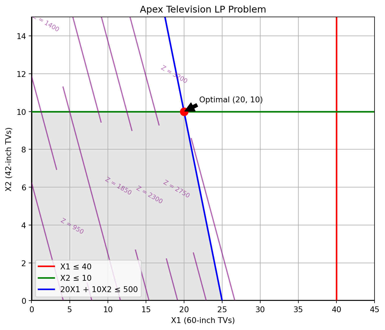
8.4 Visualization of the Apex Television Problem

Let’s visualize the solution to better understand the constraints and optimal point:

Code

import numpy as np
import matplotlib.pyplot as plt

# Create figure and axes
fig, ax = plt.subplots(figsize=(7, 6))

# Define the boundaries of the plot
x1_range = np.linspace(0, 45, 100)
x2_range = np.linspace(0, 15, 100)
X1, X2 = np.meshgrid(x1_range, x2_range)

# Plot the constraints
ax.plot(x1_range, np.zeros_like(x1_range), 'k-', lw=2)  # X2 = 0
ax.plot(np.zeros_like(x2_range), x2_range, 'k-', lw=2)  # X1 = 0
ax.plot(np.ones_like(x2_range) * 40, x2_range, 'r-', lw=2, label='X1 ≤ 40')  # X1 = 40
ax.plot(x1_range, np.ones_like(x1_range) * 10, 'g-', lw=2, label='X2 ≤ 10')  # X2 = 10
ax.plot(x1_range, (500 - 20 * x1_range) / 10, 'b-', lw=2, label='20X1 + 10X2 ≤ 500')  # Work hours

# Shade the feasible region
x1_vertices = [0, 0, 20, 25]
x2_vertices = [0, 10, 10, 0]
ax.fill(x1_vertices, x2_vertices, alpha=0.2, color='gray')

# Mark the optimal solution
ax.plot(20, 10, 'ro', markersize=10)
ax.annotate('Optimal (20, 10)', xy=(20, 10), xytext=(22, 10.5),
            arrowprops=dict(facecolor='black', shrink=0.05))

# Add objective function contour
Z = 120 * X1 + 80 * X2
contours = ax.contour(X1, X2, Z, levels=np.linspace(500, 3200, 7), alpha=0.6, colors='purple')
plt.clabel(contours, inline=True, fontsize=8, fmt='Z = %.0f')

# Set plot limits and labels
ax.set_xlim(0, 45)
ax.set_ylim(0, 15)
ax.set_xlabel('X1 (60-inch TVs)')
ax.set_ylabel('X2 (42-inch TVs)')
ax.set_title('Apex Television LP Problem')
ax.grid(True)
ax.legend()

plt.tight_layout()
plt.show()

9 Summary

Linear Programming is a powerful optimization technique with wide applications in supply chain management and operations. These skills provide a foundation for more advanced optimization models that we’ll explore in future modules, including network flow models, facility location problems, and integer programming.

10 Exercises

10.1 Production Planning

A manufacturing plant produces two types of products: standard and deluxe. Each standard product requires 4 hours of machining time and 2 hours of assembly time. Each deluxe product requires 6 hours of machining time and 3 hours of assembly time. The plant has 240 hours of machining time and 120 hours of assembly time available per week. The profit is $7 per standard product and $10 per deluxe product.

Formulate this as an LP model and solve it using both Excel Solver and Python with Gurobi to determine the optimal production levels.

Reuse

CC BY-NC-ND 4.0